Iced tutorial
Contents
Note
Doctest Mode
The code-examples in the above tutorials are written in a python-console format. If you wish to easily execute these examples in IPython, use:
%doctest_mode
in the IPython-console. You can then simply copy and paste the examples directly into IPython without having to worry about removing the >>> manually.
What is iced?
iced is a python package that contains normalization techniques for Hi-C data.
It is included in the HiC-pro pipeline, that processes data from raw fastq
files to normalized contact maps. Eventually, iced grew bigger than just being a
normalization packages, and contains a number of utilities functions that may
be useful if you are analyzing and processing Hi-C data.
If you use iced, please cite:
HiC-Pro: An optimized and flexible pipeline for Hi-C processing. Servant N., Varoquaux N., Lajoie BR., Viara E., Chen CJ., Vert JP., Dekker J., Heard E., Barillot E. Genome Biology 2015, 16:259 doi:10.1186/s13059-015-0831-x http://www.genomebiology.com/2015/16/1/259
Working with Hi-C data in Python
Hi-C data boils down to a matrix of contact counts. Each row and columns
corresponds to a genomic window, and each entry to the number of times these
genomic windows have been observed to interact with one another. Python
happens to be an excellent language to manipulate matrices, and iced
leverages a number of scientific packages that provides nice and easy-to-use
matrix operation.
Note
If you are not familiar with numpy and python, we strongly encourage to follow the short tutorial of the scipy lecture notes
Loading an example dataset
iced comes with a sample data set that allows you to play a bit with the
package. The sample data set included corresponds to the first 5 chromosomes
of the budding yeast S. cerevisiae. In the following, we start a Python or
IPython interpreter from our shell and load this data set. Our notational
convention is that $ denotes the shell prompt while >>> denotes the
Python interpreter prompt:
$ python
>>> from iced import datasets
>>> counts, lengths = datasets.load_sample_yeast()
A data set in iced is composed of an N by N numpy.ndarray counts and a
vector of lengths that contains the number of bins per chromosomes. For
our sample data, the vector lengths is an ndarray of length 5, underlying
we have here 5 chromosomes:
>>> print(len(lengths))
5
The contact map counts should be squared and symmetric. The shape should
also match the lengths vector:
>>> print(counts.shape)
(350, 350)
>>> print(lengths.sum())
350
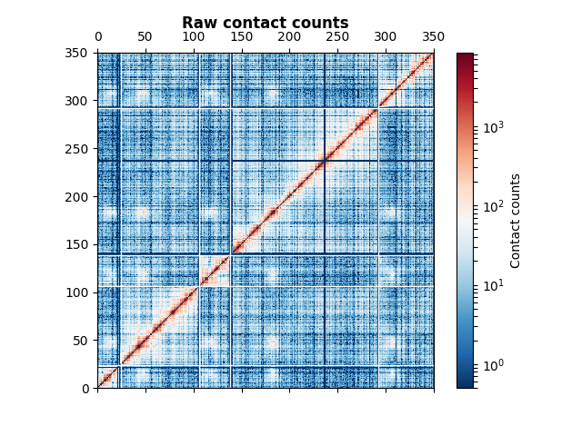
The counts matrix is here of size 350 by 350.
You’ve successfully loaded your first Hi-C data! The corresponding image is the following.
Normalizing a data set with ICE
Now that we have some data loaded, let’s proceed to normalizing it. There are two normalization algorithms implemented in iced: ICE and SCN. ICE is the most widely used normalization technique on Hi-C data, so this is the one we will showcase.
ICE is based on a matrix balancing algorithm. The underlying assumptions are
that the contact map suffers from biases that can be decomposable as a product
of regionale biases:  , where
 is the raw contact counts between loci
  and
and  ,
,
 the normalized contact counts, and
  the bias
vector.
the bias
vector.
Normalizing the data is as simple as follows
>>> from iced import normalization
>>> normed = normalization.ICE_normalization(counts)
But the estimation of the bias vector can be severely problematic in low coverage regions. In fact, if the matrix is too sparse, the algorithm may not converge at all! To avoid this, Imakaev et al recommend filtering out a certain percentage of rows and columns that interact the least. This has to be performed prior to applying the normalization algorithm:
>>> from iced import filter
>>> counts = filter.filter_low_counts(counts, percentage=0.04)
>>> normed = normalization.ICE_normalization(counts)

How about cancer data sets? LOIC and CAIC
The last section discusses normalizing Hi-C data using ICE. This method is not adapted to normalize cancer data sets: several of the assumptions made do not hold in the presence of copy number variation.
iced proposes two methods for normalizing data sets with copy number
variations:
LOIC, to preserve enrichment in interactions due to copy number variationsCAICto remove copy number variation effects in the contact count matrix.
Two examples are available in the gallery, showcasing how to use LOIC
and CAIC with ice.