mplot3d example code: lorenz_attractor.py

(Source code, png, pdf)

'''
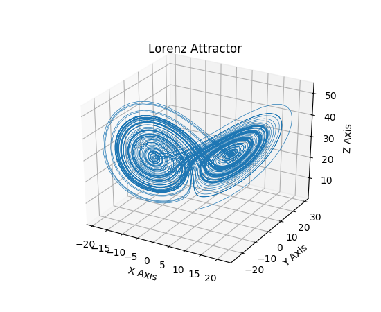
Plot of the Lorenz Attractor based on Edward Lorenz's 1963 "Deterministic
Nonperiodic Flow" publication.
http://journals.ametsoc.org/doi/abs/10.1175/1520-0469%281963%29020%3C0130%3ADNF%3E2.0.CO%3B2

Note: Because this is a simple non-linear ODE, it would be more easily
      done using SciPy's ode solver, but this approach depends only
      upon NumPy.
'''

import numpy as np
import matplotlib.pyplot as plt
from mpl_toolkits.mplot3d import Axes3D


def lorenz(x, y, z, s=10, r=28, b=2.667):
    '''
    Given:
       x, y, z: a point of interest in three dimensional space
       s, r, b: parameters defining the lorenz attractor
    Returns:
       x_dot, y_dot, z_dot: values of the lorenz attractor's partial
           derivatives at the point x, y, z
    '''
    x_dot = s*(y - x)
    y_dot = r*x - y - x*z
    z_dot = x*y - b*z
    return x_dot, y_dot, z_dot


dt = 0.01
num_steps = 10000

# Need one more for the initial values
xs = np.empty((num_steps + 1,))
ys = np.empty((num_steps + 1,))
zs = np.empty((num_steps + 1,))

# Set initial values
xs[0], ys[0], zs[0] = (0., 1., 1.05)

# Step through "time", calculating the partial derivatives at the current point
# and using them to estimate the next point
for i in range(num_steps):
    x_dot, y_dot, z_dot = lorenz(xs[i], ys[i], zs[i])
    xs[i + 1] = xs[i] + (x_dot * dt)
    ys[i + 1] = ys[i] + (y_dot * dt)
    zs[i + 1] = zs[i] + (z_dot * dt)


# Plot
fig = plt.figure()
ax = fig.gca(projection='3d')

ax.plot(xs, ys, zs, lw=0.5)
ax.set_xlabel("X Axis")
ax.set_ylabel("Y Axis")
ax.set_zlabel("Z Axis")
ax.set_title("Lorenz Attractor")

plt.show()

Keywords: python, matplotlib, pylab, example, codex (see Search examples)